
|
RTSDS |

|
A Platform for Real Time Simulation of Dynamic Systems By Isaac D. T. de Souza, Sérgio N. Silva, Rafael Teles and Marcelo A. C. Fernandes
|
|
RTSDS |
|
A Platform for Real Time Simulation of Dynamic Systems By Isaac D. T. de Souza, Sérgio N. Silva, Rafael Teles and Marcelo A. C. Fernandes
Validation of the proposed system involved the development of a prototype (illustrated in Figure 1) with M = 2 DAMs (DAM-1 and DAM-2) and N = 1 SGM (SGM- 1). The MCM was implemented using the Intel DN2800MT Mini-ITX platform with the Linux operating system (distribution: Ubuntu 13.10), and the DAMs and SGMs were implemented in microcontrollers. DAM-1 utilized an Atmel ATmega 2560 processor with Arduino Mega 2560 development kit, DAM-2 used an Atmel ATmega 328p procesor with Arduino Uno development kit, and the SGM utilized a Cypress PSOC 3 CY8C38 processor with PSOC CY8CKIT-001 kit. Communication between the two DAMs and the MCM was accomplished using the USART protocol (Universal Synchronous and Asynchronous Serial Receiver and Transmitter) at a rate of R1 = 9.6 kbps, and communication between the SGM and the MCM was by means of the USB (Universal Serial Bus) protocol, at a rate of R2 = 1 Mbps.
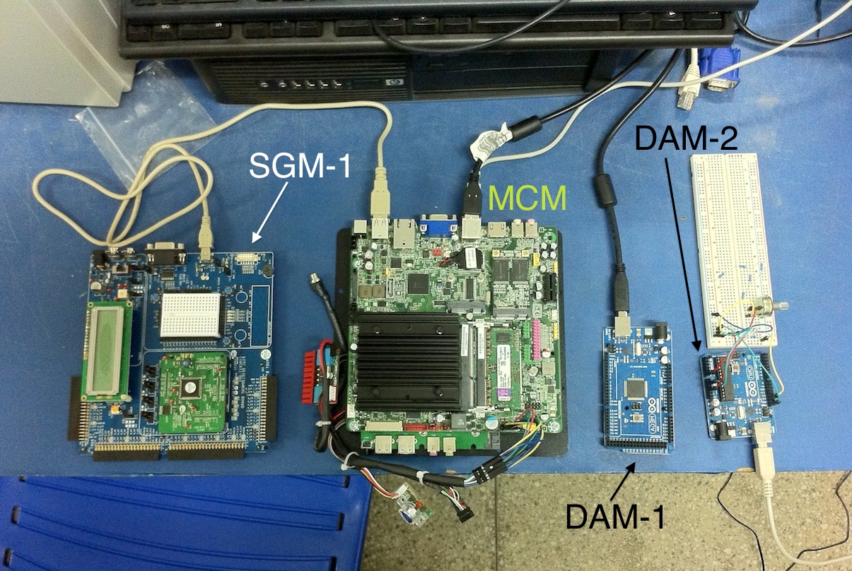
Figure 1: Prototype RTSDS composed of a MCM (Intel DN2800MT Mini-ITX), two DAMs (Arduino Mega 2560 kit), and an SGM (PSOC CY8CKIT-001 kit).
The main application of the MCM in the prototype was implemented with only one available ODS. This dynamic system is illustrated in Figure 8, and the results are presented in the next section. The real-time simulation involved a tank of water coupled to a pump (see Figure 8). The pump with constant flow, qm(t), is coupled to an input valve with continuous control, Ve(t), generating a tank input flow of qe(t). The tank output valve also possesses a continuous control, Vo(t), and the flow after this valve is given by qs(t). The level of water in the tank is characterized by the n(t) variable. In this case, the ODS (Figure 9) possesses two inputs, P = 2, controlling the input valve, Ve(t), and the output valve, Vo(t), and one output, H = 1, which is the water level in the tank, n(t). The system of differential equations associated with the ODS can be expressed by
\[\begin{equation} f(t) = \left \{ \begin{array}{l} q_e(t) - V_o(t)q_s(t)= A\frac{d n(t)}{d t} \\ q_e(t)=q_m(t)V_e(t) \\ q_s(t) = a\sqrt{2gn(t)} \end{array} \right. \end{equation}\]
where qm(t), A, g, and a are the set of adjustable parameters, M, of the ODS, representing the pump flow (cm2 = s), the transverse section of the tank (cm2), the gravitational force (m2 = s), and the transverse section of the tank output tube (cm2), respectively.
The dynamic system was simulated in real time, employing the Euler method for ODE resolution (the MethodODE variable), which is a simple but effective method for the dynamic system represented by Equation 1. In this method Equation 1 can be rewritten as
\[\begin{equation} n(t) = \left \{ \begin{array}{l} z(t) \text{ for } z(t) < n_{max}\\ n_{max} \text{ for } z(t) \geq n_{max} \end{array} \right. \end{equation}\]
where nmax is the maximum water level in the tank and
\[\begin{equation} z(t) = n_0 + \int_{t_0}^{t}g\left(s,n(s)\right) d s, \, t>t_0 \text{ e } n_0 \geq 0, \end{equation}\]
where n0 is the initial condition of the tank level and g (s, n(s)) is expressed as
\[\begin{equation} g\left(s,n(s)\right) = \frac{1}{A}\left(q_m(s)V_e(s) - V_o(s)a\sqrt{2gn(s)} \right). \end{equation}\]
The Euler method approximates the integral, presented in equation 3, by the area of a rectangle whose base has length \(\Delta\)t, in other words,
\[\begin{eqnarray} z(t+\Delta t) & = &n_0 + \int_{t_0}^{t}g\left(s,n(s)\right) d s + \int_{t}^{\Delta t}g\left(s,n(s)\right) d s \nonumber \\ & \approx & z(t)+g\left(t,n(t)\right) \times \Delta t \end{eqnarray}\]
where \(\Delta t\) is the step of the Euler method. For RTSDS, \(\Delta t\) is the run time of the ST, \(t_s = \Delta t\). Thus, the resolution method implemented in the prototype can be expressed as
\[\begin{equation}\label n(t+t_s) = \left \{ \begin{array}{l} v(t) \text{ for } v(t) < n_{max}\\ \\ n_{max} \text{ for } v(t) \geq n_{max} \end{array} \right. \end{equation}\]
where,
\[\begin{equation} v(t) = \left(\frac{1}{A}\left(q_m(t)V_e(t) - V_o(t)a\sqrt{2gn(t)} \right)\right) \times t_s. \end{equation}\]
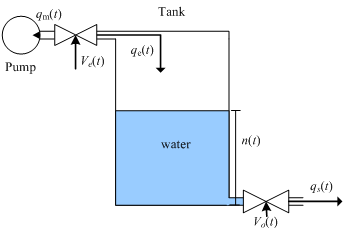
Figure 2: Dynamic system simulated in real time using the prototype.
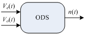
Figure 3: Instantiated ODS object composed of two inputs, P = 2, (control of the input valve, Ve(t), and control of the output valve, Vo(t)), and one output, H = 11, (level of water in the tank, n(t)).
The control signal of the input valve actuator, \(V_e(t)\), can have values of between 0 and 1 in the ODS. In order to represent a more real situation, the external signal, \(x_{11}(t)\), associated with \(V_e(t)\) consists of a digital signal with a fixed frequency and a pulse width that can be varied between 0% and 100% (pulse-width modulation, PWM). Hence, the DAM-1, using an embedded ADAM (set C of codes) in the ATmega 2560, can recognize the PWM pulse width \(x_{11}(t)\) in real time, and convert it to a value of between 0 and 1, which is transmitted to the MCM via the USART protocol at a rate of \(R_1\) = 9.6 kbps. The resolution of the value associated with \(V_e(t)\) in conversion of the PWM signal was 8 bits (\(b_1=8\)), in order to simplify the transmission process, resulting in a transmission time of 0.83 ms. The embedded application in the DAM-1 had an execution time of around 110 ms, due to the frequency of 100 Hz utilized in the PWM.
In the case of the control signal associated with the outlet valve actuator, \(V_o(t)\), the ODS also operates with values of between 0 and 1. However, in order to differentiate this case from the preceding case, the external signal, \(x_{21}(t)\), associated with \(V_o(t)\), has an amplitude that is variable between 0 and 2.5 volts. In this way, the DAM-2, using an embedded ADAM (set C of codes) in another ATmega 2560, recognizes the amplitude of the signal \(x_{21}(t)\) in real time, and converts it to a value of between 0 and 1 for transmission to the MCM by means of the USART protocol at a rate of \(R_1\) =9.6 kbps. The resolution of the value associated with \(V_o(t)\) in the analog/digital conversion was 8 bits (\(b_1\)=8$), resulting in a transmission time of 0.83 ms. The embedded application in the DAM-2 had an execution time of around 20 ms.
Finally, the output of the simulated dynamic system, $n(t)$, which represents the level in the tank, was associated with an analog signal, $s_{11}(t)$, in SGM-$1$. In this case, the embedded ASGM (set D of codes) in the SGM-$1$ simulates an analog level sensor of a type widely used in industry, with output values of between $0$ and $1$ volt. A resolution of $8$ bits was used for the value of the level output, $n(t)$, with a transmission rate of $1$ Mbps (via USB protocol) between the MCM and SGM-$1$, resulting in a transmission time of around $8 \, \mu \text{s}$. The resolution of the digital/analog converter in SGM-$1$ was $8$ bits, and the execution time of the ASGM was approximately $1\, \text{ms}$.
Table 1 summarizes the times estimated for the DAMs and SGMs, based on the variables presented in Equation 2 from the architecture section. From these values and the response time of the dynamic system, $t_r$, it is possible to estimate the value of $t_s$ and calculate the sampling time of the system, $t_a$.
| Times | DAM-1 | DAM-2 | SGM-1 | MCM | Selected |
|---|---|---|---|---|---|
| $t_{MAD}$ | 110 ms | 20 ms | - | - | 110 ms |
| $t_1$ | 0.83 ms | 0.83 ms | - | - | 0.83 ms |
| $t_{MGS}$ | - | - | 1 ms | - | 1 ms |
| $t_2$ | - | - | $8 \, \mu \text{s}$ | - | $8 \, \mu \text{s}$ |
$t_{DAT}$ $(t^w_{DAT}=100\, \mu \text{s})$ |
- | - | - | $200 \, \mu \text{s}$ | $200 \, \mu \text{s}$ |