
|
RTSDS |

|
A Platform for Real Time Simulation of Dynamic Systems By Isaac D. T. de Souza, Sérgio N. Silva, Rafael Teles and Marcelo A. C. Fernandes
|
|
RTSDS |
|
A Platform for Real Time Simulation of Dynamic Systems By Isaac D. T. de Souza, Sérgio N. Silva, Rafael Teles and Marcelo A. C. Fernandes
Figure 1 shows a block diagram of the architecture of the RTSDS. The main control module (MCM) is coupled to a set of M data acquisition modules (DAMs) and N signal generation modules (SGMs). The function of the MCM is to control, manage, and configure the real-time simulation platform, and it is also responsible for the entry and retrieval of data by the user.
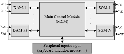
Figure 1: Physical architecture of the RTSDS.
The DAMs and SGMs are auxiliary hardware whose function is to receive and generate signals related to the dynamic system to be simulated by the MCM. In practice, the DAMs and SGMs can be implemented by a variety of hardware platforms, such as digital signal processors, microcontrollers, and other devices possessing digital and/or analog inputs and outputs. As shown in Figure 1, each m-th DAM can include L digital and/or analog inputs, and each n-th SGM is characterized by K digital and/or analog outputs. Each RTSDS must possess at least one DAM and one SGM.
The main control module is responsible for configuring and implementing the simulation of the chosen dynamic system. The MCM performs its task by means of an embedded application called the main application (MA), which will be described in the following sections. In addition to the MA, the MCM must possess a set of integrated interfaces and communication protocols in order to achieve communication with the DAMs and SGMs. The RTSDS platform does not demand any specific communication protocol, although the transmission rate R (in bps) is an important factor in the functioning of a real-time simulator, especially in the case of fast-response dynamic systems.
The DAMs are hardware connected to the MCM by means of a data communication protocol transferring bits at a rate of R1 bps. Each m-th DAM can comprise L inputs (analog and/or digital), and is responsible for capturing signals from the external environment that will be used by the real-time simulator executed in the MCM. The DAMs utilize an embedded software system, called the application DAM (ADAM). There is a different ADAM for each type of driver and actuator associated with the dynamic system to be simulated. The ADAM is responsible for transforming the L external signals connected to the m-th DAM into real values, and transmitting them to the MCM. The l-th input signal of the m-th DAM is expressed by xml(t), and depending on the driver may be a variable amplitude and/or frequency analog signal, or a variable frequency and/or pulse width digital signal.
These modules are hardware platforms responsible for the generation of signals associated with the outputs of the dynamic system simulated in the MCM. Similar to the DAMs, the SGMs are comprised of K outputs (analog and/or digital), communicate with the MCM by means of a data communication protocol at a rate of R2 bps, and employ an embedded software system called the application SGM (ASGM), which converts the simulation data received from the MCM into external analog and/or digital signals. For each type of sensor to be simulated in the dynamic system, there is a different ASGM that converts the output information according to the instrumental characteristics of the sensor in question. The k- th output signal of the n-th SGM is expressed as snk(t), and depending on the type of sensor may be an analog signal of variable amplitude and/or frequency, or a digital signal with variable frequency and/or pulse width [15].
Figure 2 illustrates the logical architecture of the RTSDS, where an application located in the MCM, here known as the main application (MA), instantiates a class of software called the object dynamic system (ODS). An ODS represents the dynamic system to be simulated in real time, and is composed, amongst others, of 8 principal attributes expressed by {P;H; f(t);M; C;D; MethodODE; ta}, where
The RTSDS possesses a database, located in the MCM, composed of various ODSs that can be easily inserted by means of the MA.
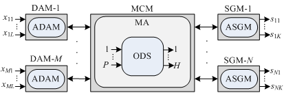
Figure 2: Logical architecture of the RTSDS.
The execution of the real-time simulation of an ODS, in the MCM, is achieved using three threads working collaboratively. These are the data acquisition thread (DAT), the simulation thread (ST), and the time control thread (TCT). The function of the DAT is to update all the P inputs of the dynamic system under simulation, reading all the input buffers associated with the data connections between the MCM and the DAMs. The P input variables are shared between the data acquisition and simulation threads. The ST updates the H output variables and executes the ODE numerical resolution method (defined by the MethodODE variable) in the system of equations, f(t), in order to update the states of the dynamic system. The execution of the simulation thread is controlled by the TCT, which uses semaphore logic to regulate the execution time of the ST to a fixed value, ts, so that the resolution method always occurs at fixed intervals. The use of a fixed interval, ts, is not essential in numerical resolution methods, but is fundamental for parameterization of the simulation platform, which must have a sampling time, ta, that is much smaller than the response time, tr, of the dynamic system to be simulated. In other words, the simulation process must respect the restriction
\[\begin{equation}\label{EqR} t_a << t_r \end{equation}\]
Figure 3 illustrates the functional relationships between the DAT, ST, and TCT.
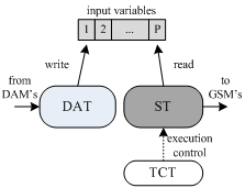
Figure 3: Relationships between the DAT, ST, and TCT.
The Figures 4, 5 and 6 detail the finite automata associated with the threads DAT, TS and TCT, respectively. The DAT (Figure 4) scans all communication interfaces buffers with DAMs and updates the P input variables of ODS (Figure 3). The DAT is asleep in a predetermined fixed time, tw DAT , to minimize collision problems in the input variables update (write operation), since they are shared with the ST. The finite automata of ST (detailed in Figure 5) waiting for the semaphore resource update (by TCT) to send the output variables to SGMs and then run the ODS. Finally, Figure 6 shows, by finite automata, the operation of TCT which controls the insertion of the semaphore resource. The resource addition is done every, ts, seconds to ensure the run time of the ODS. The finite automata shown in Figure 6 also details a system synchronization (Using the variables da and d) that adjusts the run time in ts.
The codes of the set C associated with an ODS act as transducers between the external input signal (which can be digital or analog) and one of the P inputs of the dynamic system. Each ODS has a one to many relationship with the DAMs, and if necessary, can use all the M DAMs available. The decision of which and how many DAMs will be used by the ODS is made off-line by means of configuration parameters, with the objective of customizing the performance of the system in order to reduce the sampling time, ta. An important point is that the DAMs can simulate the effect of real drivers and actuators, for example the commercial drivers that work with signals possessing variable frequency and pulse width.
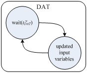
Figure 4: Finite automata associated with DAT.
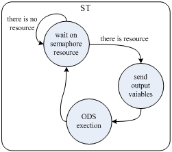
Figure 5: Finite automata associated with ST.
Similar to the DAMs, the role of the set D of codes related to the ODS is to act as transducers between the outputs of the dynamic system and the external signals (digital and/or analog) to be generated. Each ODS also has a one to many relationship with the SGMs, and can if necessary utilize all N SGMs associated with the RTSDS. The configuration of which and how many SGMs will be used during the real-time simulation process is configured off-line, as for the DAMs. The SGMs can also simulate the responses of real commercial sensors with variable frequency, amplitude, or pulse width.
The simulation of drivers and sensors (using the DAMs and SGMs, respectively) coupled to the dynamic system differentiates the proposed platform, with the simulation process becoming closer to the real case. This benefit is especially important in the development and validation of embedded control of dynamic systems. Future work will consider the optimization of algorithms for the automatic allocation of DAMs and SGMs to the MCM.
After instantiation of an ODS, the sampling time, ta, can be expressed by
\[\begin{equation}\label{EqTempo} t_a = t_{DAM} + t_{1}+t_{DAT}+t_{s}+t_{2}+t_{SGM} \end{equation}\]
where tDAM is the fastest processing time associated with all the DAMs utilized by the MCM, t1 is the time corresponding to the slowest rate of transfer (in bps) between the MCM and all the DAMs utilized, tDAT is the time taken by the DAT to read the information received by all the DAMs, ts is the time required for execution of the ST, t2 is the slowest transfer time (in bps) between the MCM and the SGMs, and tSGM is the fastest processing time associated with all the SGMs utilized by the MCM. The transmission time, t1, between a DAM and the MCM can be described by
\[\begin{equation} t_1=\frac{b_1}{R_1} \end{equation}\]
where b1 is the resolution (in bits) of the value to be transmitted. Similarly, the transmission time between the MCM and the SGM can be expressed by
\[\begin{equation} t_2=\frac{b_2}{R_2} \end{equation}\]
where b2 is the resolution (in bits) of the value transmitted.
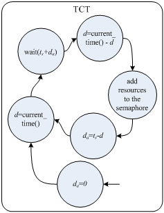
Figure 6: Finite automata associated with TCT.